
Simulation as a Proof Method for Data Refinement
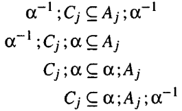
In previous chapter, we have to verify that an infinite number of inclusions should hold to prove the correctness of specific data refinement, shown as following:
Consequently it does not yield an effective proof method.
This chapter has the following main concept:
- simulation
- abstraction relation
- data invariant
- Proofs are carried out in predicate logic
- How to express abstraction relations within predicate logic
- normal variables: unaffected by the data refinement step
- representation variables: affected by that step
Simulation
The previous criterion is infinite inclusions. At the same time, it is a global criterion. Simulation is a local criterion that result in a finite number of verification conditions, and hence providing an effective proof method.
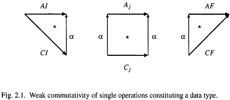
In the middle of above picture, the following inclusions will be generated.
Such that, we have four ways to define proof method in which the verification conditions have the form of inclusions between relations.
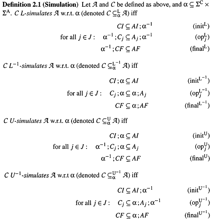
It is finite conditions, since the index set J is assumed to be finite. The four notions above are essentially different. This is because the relation $\alpha$ is not necessarily total and functional. If it is, the four notions are coincide.
Def. 2.1 raises the following two questions.
- When do these notions of simulation imply the global criterion of data refinement? This question concerns the soundness of these methods,
- Assuming that $\mathcal{C}$ is a data refinement of $\mathcal{A}$, can this fact always be proven using one or more of these notions of simulation? This question concerns the completeness of these methods.
Soundness and (In)completeness of Simulation
L-simulation is indeed soundness.
Lemma 2.2 (L-simulation implies data refinement) Let $\mathcal{A}$ and $\mathcal{C}$ be compatible data types and let $\alpha$ be an abstraction relation such that $\mathcal{C}\subseteq_{\alpha}^{\text{L}}\mathcal{A}$, Then $\mathcal{C}$ is a data refinement of $\mathcal{A}$.
Unfortunately, it is incompleteness. I.e., given that a data type is a data refinement of another one, as defined above, that result cannot always be proven using L-simulation in the sense of Def. 2.1.
Data Invariants
In previous discussion, an abstract relation is used in simulation. We known this relation is neither total nor functional.
Relations vs. Functions
General relations are sometimes indispensable.
Example 2.4 shows a total and functional abstraction relation: elts on linear list. In example 2.5, using a specific example to show representation variables(in the case sum and num) and normal variables($x$ and $av$ in this case), then, in the example the abstraction relation is non-functional.
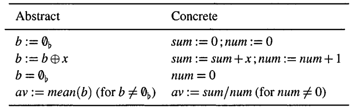
The corresponding abstraction relation $\alpha$ is defined by $(\sigma, \tau) \in \alpha$ iff
\[\sigma(av) = \tau(av)\wedge \sigma(x)=\tau(x) \wedge \Sigma_b(\tau(b)) = \sigma(sum)\wedge \#(\tau(b)) = \sigma(num)\]Where for the same $\sigma$, there is more than one $\tau$ corresponding to satisfy the relation. So, the relation is non-functional.
Data invariant (characterizing the reachable values in a data type) solve one of the problems associated with converting abstraction relations into abstraction functions. It can be used to identify a subspace on which $\alpha$ is total.
representation invariant: A representation invariant consists of two parts: a data invariant of the concrete data type and an abstraction relation between concrete and abstract data.
Abstraction Relations and Normal Variables
How shall we prove data refinement in these examples?
In previous chapter, when defining the data refinement, a data type $\mathcal{A}$ involves operation on representation variables and normal variables. Since normal variables is unaffected by data refinement step, there should be no need to check verification conditions for normal operations.
Two methods treat to representation variables and normal variables:
- VDM: only represented operations are considered, disregarding normal operations
- Reynolds’ method: normal operations may occur.
I am still confused for syntactic and semantics method.
In this section, the main notion is below, by my personal understanding:
Because the normal variable is not change by refinement steps, in the abstraction relation, just representation variable relation is needed. If the relation between representation variables in both level is given $\tilde{\alpha} \subseteq \Sigma_\text{C} \times \Sigma_\text{A}$. Then abstract relation $\alpha$ is defined below:
\[\alpha = \{((\sigma, \sigma_\text{C}), (\sigma, \sigma_\text{A}))\in \Sigma^\text{C} \times \Sigma^\text{A} | (\sigma_\text{C}, \sigma_\text{A})\in\tilde{\alpha}\}\]Where $\sigma \in \Sigma^{\text{N}}$.
Before we define the abstract relation, we need to define operations in both level:
\[op_\text{C} = \{((\sigma, \sigma_\text{C}), (\tau, \sigma_\text{C}))\in \Sigma^\text{C} \times \Sigma^\text{C} | (\sigma, \tau)\in op\}\]In abstract level:
\[op_\text{A} = \{((\sigma, \sigma_\text{A}), (\tau, \sigma_\text{A}))\in \Sigma^\text{A} \times \Sigma^\text{A} | (\sigma, \tau)\in op\}\]Where $op \subseteq \Sigma^{\text{N}} \times \Sigma^{\text{N}}$ is a given operation between states of normal variables.
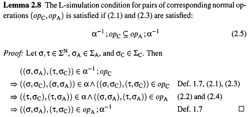
If all above restriction in this section is satisfied, the below Lemma is hold.
Towards a Syntactic Characterization of Simulation using Predicate Logic
In Example 2.9, the author said this example illustrates the difference between the role of normal variables in the semantics and syntactic versions of an abstraction relation. But I am still confused in this point.
I want to know what is syntactic or semantics form of abstraction relation. However, I will try to explain the notion by myself personal understanding:
Reconsider Example 1.4 the relation in both semantics and syntactic form is illustrated below:
- syntactic form: $elts(l) = U$
- semantics form:
Example 2.10 wants to explain this question:
Since we use the same symbol to represent normal variable in both level, when normal variables included in return expression at both level may be unequal.
Two semantics functions $\mathcal{A}\llbracket . \rrbracket \subseteq \Sigma^\text{C} \times \Sigma^\text{A}$ and $\mathcal{P}\llbracket . \rrbracket\subseteq \Sigma^\text{A/C} \times \Sigma^\text{A/C}$.
- $\mathcal{A}\llbracket . \rrbracket$: assigns meanings in terms of binary relations on states to syntactic representations of abstraction relation.
- $\mathcal{P}\llbracket . \rrbracket$: assigns meanings in terms of binary relations on states to syntactic representations of operations.
Meanwhile, in this example, we have a simple-minded set-up syntactic which cannot discover the inconsistent but semantics can. We have to formulate a proof method for data refinement which is based on predicate logic and which is sound to avoid semantics checking.
When we add an extra condition to make the proof method based on syntactic consistent, example 2.11 using this method with an extra condition to prove data refinement in Example 2.5.
Subsection “A first encounter with Reynolds’ method” illustrates an application of the method in Example 1.1 to get a concrete program from an abstract one following 4 steps R1 $\rightarrow$ R4.
Further, in subsection “A first encounter with VDM”, VDM method is used to achieve the same purpose in previous subsection.